Machine learning models in computer vision are being utilised in many real-world applications such as self-driving cars, facial recognition, cancer detection, and even next-generation stores to track which things consumers take off the shelf so their credit card may be charged when they leave.
And a few years ago, getting wrong predictions from such a machine learning model used to be the norm which now is an exception. As machine learning models are deployed in real-world settings rather than being tested in a laboratory setting, security risks caused by model flaws have become a major concern.
The goal of this article is to describe how machine learning models can be readily deceived by malevolent actors or adversarial examples, causing them to make incorrect predictions. We will examine how adversarial examples are features rather than flaws once we are acquainted with the basic understanding of the underlying topics.
What are Adversarial examples?
Adversarial examples are harmful inputs created with the intent of fooling a machine learning model. These are a sample of input data that has been very slightly manipulated in order to induce machine learning to misclassify it.
An example should assist to solidify the concept.

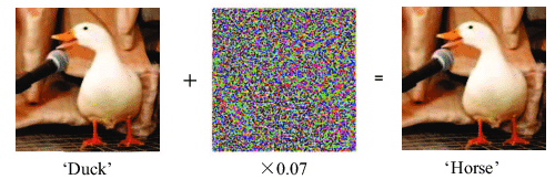
The two photos above (the leftmost and the rightmost) are indistinguishable to the human eye. The picture on the left is one of the clean images, while the image on the right is a little variation of the first, made by including the noise vector in the centre image.
The model predicts that the first image is of a Duck, as expected. The second, on the other hand, is projected to be a Horse (with a high degree of certainty).
How to Generate Adversarial Examples?
Adversarial examples are created by starting with a clean picture that the model successfully classifies and then looking for a slight perturbation that causes the new image to be misclassified by the ML model.
Assume an attacker has complete knowledge of the model they intend to attack. This basically means that the attacker may compute the model's loss function J(θ, X,y), where X is the input picture, y is the output class, and are the internal model parameters. For classification algorithms, this loss function is often the negative loss likelihood.
There are various methods to generate adversarial examples, each method indicating a distinct balance between computing cost and success rate. All of these strategies aim to maximize the change in the model loss function while minimizing the perturbation of the input picture. The greater the dimension of the input picture space, the easier it is to develop adversarial examples that are visually indistinguishable from clean images.
Adversarial Training
As the title of the article suggests - “Adversarial Examples Are Not Bugs, They Are Features”. The best way to handle the adversarial examples by our machine learning model is to train the model itself with the adversarial examples. This method is commonly referred to as adversarial training.
When training the model, adversarial examples are created and used. Intuitively, if the model observes hostile cases during training, its performance for adversarial examples created in the same way will be better at prediction time. In an ideal world, we would use any known attack mechanism to produce adversarial examples during training.
Adversarial training employs a modified loss function that is a weighted sum of the standard loss function on clean instances and a loss function from adversarial cases.

During training, for every batch of m clean photos, we produce k adversarial images using the network's current state. We forward propagate the network for both clean and adversarial cases and use the aforementioned algorithm to determine the loss.
However, for large datasets with high dimensionality, resilient attack techniques such as L-BFGS and the enhancements outlined in the Berkeley research are computationally prohibitively expensive. In actuality, we can only afford to adopt a rapid approach such as FGS (Fast Gradient Sign Method) or iterative FGS.
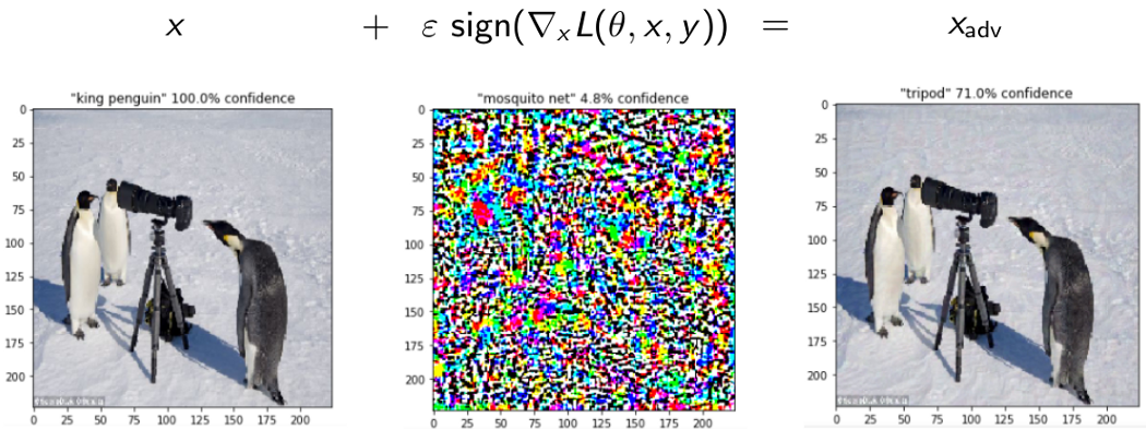
Let x represent the original picture, y the class of x, the network weights, and L(θ, x, y) the loss function used to train the network.

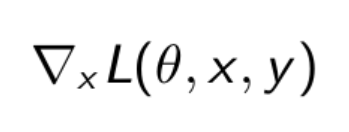
To begin, we compute the gradient of the loss function based on the input pixels. The operator is just a straightforward mathematical method for calculating the derivatives of a function based on several of its parameters. Consider it a shape matrix [width, height, channels] storing the slopes of the tangents.

As previously said, we are solely interested in the slopes' sign to determine whether we want to raise or decrease the pixel values. To guarantee that we do not move too far on the loss function surface and that the perturbation is undetectable, we multiply these signs by a very little number. This will be our perturbation.

Our final image is simply our original image with the perturbation applied.

Figure: An picture with FGSM applied on it. The original is classed as a "king penguin" with 100% certainty, whereas the disturbed one is labelled as a "tripod" with 71% certainty.
Conclusion
Attacking a machine learning model is now simpler than protecting it. If no defense strategy is used, state-of-the-art models implemented in real-world applications are readily deceived by adversarial examples, opening the door to potentially serious security vulnerabilities.
Finding new attacks and improved protection tactics is a topic for ongoing scientific research. More theoretical and empirical research is needed to improve the robustness and safety of machine learning models in real-world applications.
But as of now for handling adversarial examples, adversarial training is the most dependable protection approach, in which adversarial examples are produced and added to clean examples throughout training