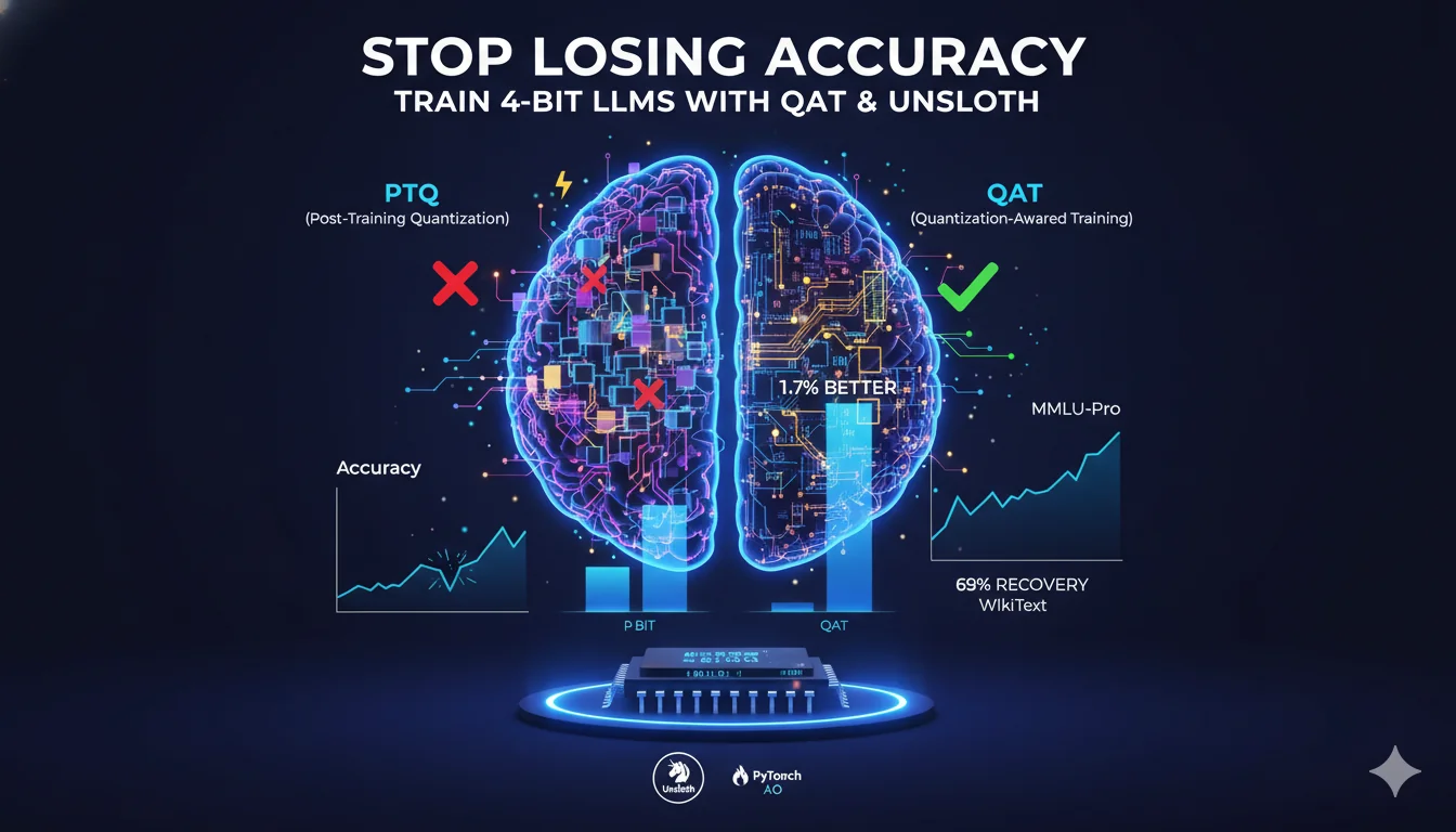
Let's be real: we've all been there. You spend days (or nights) fine-tuning a new LLM, feeling pretty good about it. Then, to make it run faster, you quantize it to 4-bit. The model's accuracy drops dramatically.
We shrink models to make them faster and cheaper to run, but it always feels like a bad trade-off: Accuracy for Speed.
The usual culprit is Post-Training Quantization (PTQ). It's the "fast and easy" method where you train your model first, then just squish it down to 4-bit afterward. The problem? The model was never built for that, and the performance hit can be painful.
But what if you could get that 4-bit speed and keep your original accuracy? Or even.. beat it?
That's what Quantization-Aware Training (QAT) is all about. Instead of squishing the model after, you make it "aware" of the 4-bit limits while it's still training.
The folks at Unsloth and PyTorch AO are the ones who really cracked this. They built the tools that make it possible.
My goal here isn't to reinvent the wheel. It's to show you how to use their work to get the same awesome results. I ran the experiment myself, fine-tuning a Qwen3-4B model, just to prove it out.
And the results are in: This stuff really works.
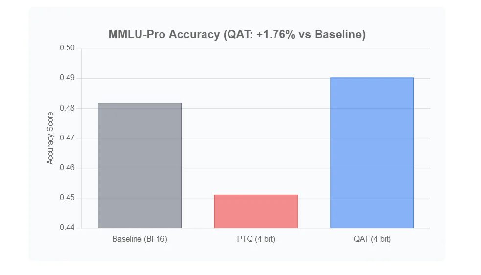
In my own tests, the QAT method recovered 69% of the accuracy on the WikiText benchmark. Even better, on MMLU-Pro test, it actually beat the original full-precision model by 1.7%.
So, let's walk through how you can do it, too.
Get ₹2,000 free credits to test your AI workloads
Sign up and complete ID verification to unlock free credits. Deploy on NVIDIA H200, H100, and L40S GPUs—no commitment required.
How Quantization Actually Works: PTQ vs. QAT
To understand why QAT is so effective, we first need to cover a few core concepts.
What is Quantization?
At its simplest, quantization is the process of reducing the precision of numbers. Our model's weights (the parameters it learned during training) are typically stored in 32-bit(FP32), or 16-bit (BF16 or FP16). Let's consider we have them in BF16.
A 16-bit number can represent over 65,000 different values. An INT4 (4-bit integer) number can only represent 16 different values.
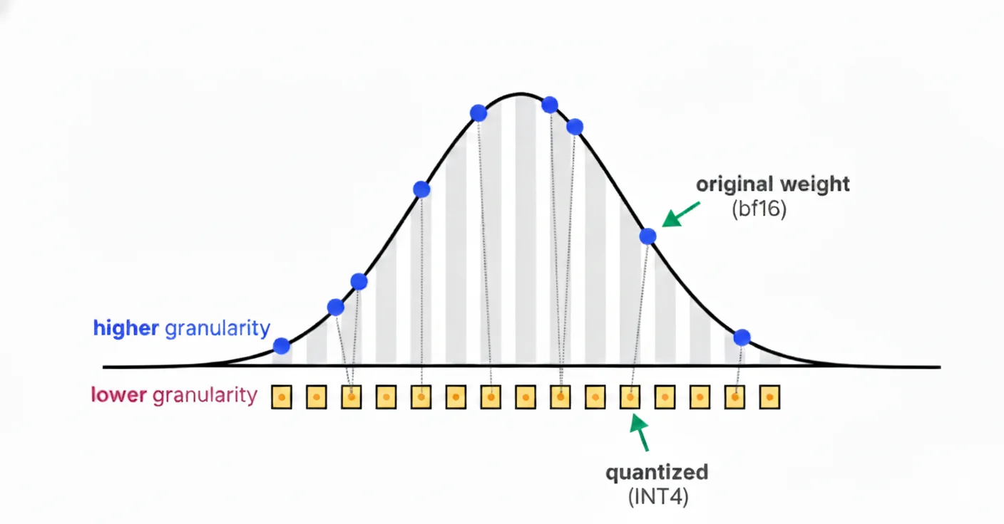 source : https://www.maartengrootendorst.com/blog/quantization/
The goal is to map the massive BF16 range to the tiny INT4 range without losing the "meaning" of the weights. We do this using two key parameters:
- Scale: A multiplier that scales the numbers up or down.
- Zero-Point: An offset that shifts the entire range.
This mapping leads to two main ways of "squishing" the numbers.
Symmetric vs. Asymmetric Quantization
- Symmetric Quantization: This method is simple and fast. It forces the range of numbers to be centered around 0. The "zero-point" is always 0.
- Analogy: Imagine a ruler where 0 must be in the exact center. If your
BF16numbers range from -100 to +100, it works perfectly. But if your numbers range from +10 to +210 (like after a ReLU activation), you "waste" half your 16 available 4-bit values representing numbers from -210 to 0 that don't even exist in your data.
- Analogy: Imagine a ruler where 0 must be in the exact center. If your
- Asymmetric Quantization: This method is more flexible and accurate. It shifts the "zero-point" to match the data.
- Analogy: This is a "sliding" ruler. For the data ranging from +10 to +210, it sets the 4-bit "0" to represent the
BF16"+10" and uses all 16 available values to cover the range up to +210. It doesn't waste any space.
- Analogy: This is a "sliding" ruler. For the data ranging from +10 to +210, it sets the 4-bit "0" to represent the
Want to learn more? For a more detailed breakdown of these concepts, check out this excellent blog post: Quantization in LLMs.
Now, let's look at when we apply these techniques.
Post-Training Quantization (PTQ)
This is the "squish it after" method. It's fast and easy, but often less accurate. Popular PTQ methods you might have heard of include AWQ and GPTQ but in this blog we are using weight-only PTQ so caliberation dataset is not needed.
- You train your model in full
BF16precision. - After training, you quantize it. For weight-only PTQ (like what we're using in our experiment), the quantization parameters (
scaleandzero-point) are determined directly from the statistics (min/max values) of theBF16weights themselves, often on a per-group basis. This means you don't need a separate calibration dataset to run through the model, which simplifies the process. - The
BF16weights are then converted into theirINT4representation.
The problem? The model was never trained to handle the rounding errors (quantization noise) this process introduces, leading to potential accuracy drops.
Quantization-Aware Training (QAT)
This is the "train it to be squished" method. It's our focus today.
With QAT, you're simulating the 4-bit errors during the fine-tuning process. The model learns to adapt its weights to compensate for this noise (the rounding errors), resulting in dramatically higher accuracy.
This is how it works on every single training step:
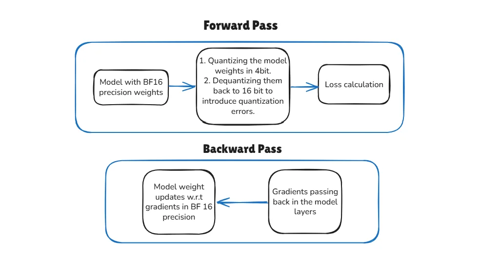
Forward Pass (Simulating the Error)
- Start: The model begins with its full-precision
BF16weights. - Simulate 4-bit Precision: This is where the magic happens, and it's a two-part process that uses the
scaleandzero-pointwe discussed.- Quantize: First, the model calculates a
scaleandzero-pointfor theBF16weights. It uses them to "squish" the weights into their 4-bit integer representation. This simulates the precision loss. - De-Quantize: It immediately uses that same
scaleandzero-pointto convert those 4-bit integers back into theBF16format.
- Quantize: First, the model calculates a
- Calculate: The forward pass (e.g., matrix multiply) is then performed using these "degraded"
BF16weights. The model is now "seeing" the rounding errors and precision loss that a real 4-bit model would have.
Backward Pass (Learning from the Error)
- Calculate Loss: The model's final output (which includes the 4-bit errors) is compared to the correct answer, and a loss is calculated.
- Pass Gradients (The "Trick"): This is the clever part. The rounding step from the forward pass isn't "differentiable"—its gradient is zero, which would stop the model from learning. QAT uses a trick called the Straight-Through Estimator (STE).
- Analogy: Think of STE as a "detour" for the gradient. On the backward pass, the gradient travels back toward the weights. When it hits the "broken" (non-differentiable)
round()function, STE simply "pretends" it's not there and directs the gradient straight through to the original weights, as if it were a simple 1-to-1 connection.
- Analogy: Think of STE as a "detour" for the gradient. On the backward pass, the gradient travels back toward the weights. When it hits the "broken" (non-differentiable)
- Update Weights: Because of STE, the gradients (which contain information about the 4-bit error) successfully reach and update the original, full-precision
BF16weights.
Over thousands of steps, the full-precision weights learn to adjust themselves. They learn to avoid "ambiguous" values that are close to a rounding boundary. In this way, they become "robust" to the 4-bit squishing process, ensuring the final 4-bit model is as accurate as possible.
The Trade-off: Slower Training for a Smarter Model
This simulation adds extra math (the quantize/de-quantize step) to every single training pass.
- The Trade-off: QAT is slower than a standard fine-tuning run. In our experiment, the QAT model took about 4 hours to train, while the standard PTQ-path model only took 2 hours.
- The Payoff: You invest more time upfront during training, but the result is a final 4-bit model with dramatically higher accuracy, as our benchmarks will show.
Quick Comparison: PTQ vs. QAT
Here's a simple table to lock in the difference.
| Feature | Post-Training Quantization (PTQ) | Quantization-Aware Training (QAT) |
|---|---|---|
| When? | After training is finished. | During the training process. |
| How? | Squishes a fully-trained model once. | Simulates 4-bit errors on every step. |
| Goal? | Speed and size reduction. | Maximize accuracy while getting speed. |
| Cost? | Very fast (seconds to minutes). | Slower (adds overhead to training). |
| Result? | Good, but almost always loses accuracy. | Excellent. Can match or beat the baseline. |
A Quick Look at Int4WeightOnlyConfig
This configuration, used for our PTQ baseline, implements grouped, asymmetric, weight-only INT4 quantization.
In our PTQ script, to create our 4-bit baseline, we used torchao's Int4WeightOnlyConfig: quant_config = Int4WeightOnlyConfig(group_size=128, ...)
What does this actually do?
-
WeightOnly: This is a crucial distinction. It only quantizes the model's weights (theLinearlayers) toINT4. The activations (the data flowing between layers) remain inBF16. This is a very common and effective PTQ method for inference speedups with minimal fuss. -
group_size=128: This is the secret to its accuracy. Instead of calculating onescaleandzero-pointfor an entire multi-million-parameter weight matrix (which is very inaccurate), it breaks the matrix into small groups of 128 numbers. It then calculates a separatescaleandzero-pointfor each tiny group directly from the weight values within that group. This is far more granular and better handles outliers, which is why "grouped" quantization is so much better than per-tensor quantization.
The Power Behind the Recovery: Unsloth and PyTorch AO

The impressive accuracy recovery and performance boost we're discussing aren't just theoretical. They're made possible by the innovative work and seamless integration provided by Unsloth and TorchAO. These are the core components of the solution that Unsloth has championed, and which we've leveraged in our experiments.
-
Unsloth: This is the high-performance framework that makes LoRA fine-tuning incredibly fast and memory-efficient. Unsloth's magic lies in its optimized kernels and its deep integration with quantization techniques. When we pass
qat_scheme = "int4"to Unsloth, it intelligently leveragestorchaounder the hood to perform the QAT loop, transforming a regular fine-tuning run into a Quantization-Aware one with minimal fuss for the developer. -
PyTorch AO (
torchao): This is PyTorch's native library for advanced quantization and optimization. It provides the robust, low-level building blocks for both PTQ and QAT. Unsloth integrates directly withtorchaoto manage the quantization process during training and conversion.
Get ₹2,000 free credits to test your AI workloads
Sign up and complete ID verification to unlock free credits. Deploy on NVIDIA H200, H100, and L40S GPUs—no commitment required.
GPU Machine Setup for Model Training (H100)
If you'd like to follow this tutorial step-by-step, you can easily rent a GPU machine tailored to your needs on the E2E Networks platform. Check the GPU pricing page for current rates. Following are the steps I followed to get my GPU instance ready for model training.
Step 1: Launching Your GPU Instance
First, let's get your GPU instance launched on the TIR platform of E2E Networks. It's a straightforward process.
-
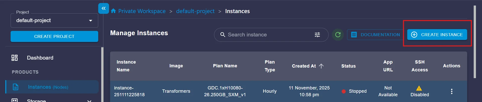
Log in to your E2E Networks account and find the Instances (Nodes) section (usually under Products in the sidebar).
-
Click the CREATE INSTANCE button.
-
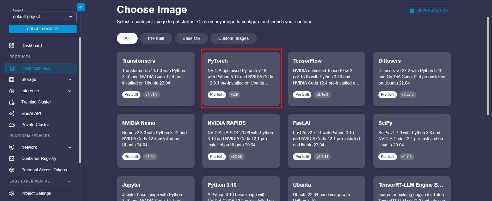
Choose Image: Head to the Pre-built tab and select the PyTorch image. This is a massive time-saver, as it comes with the NVIDIA drivers, CUDA, PyTorch, and other key tools already installed.
-
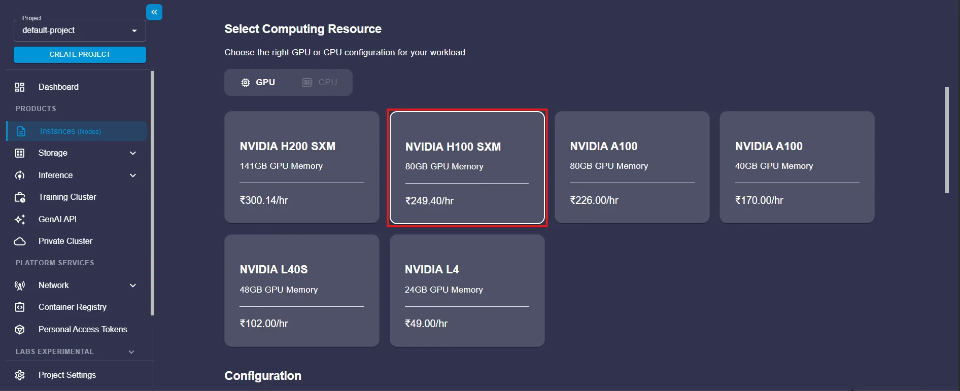
Choose a Plan: Select a GPU instance that fits your needs. For a powerful model like this, we're selecting an H100 instance, which is perfect for heavy-duty training or high-throughput inference.
-
Select Pricing: To save on costs, especially for batch jobs that don't need to run 24/7, choose the Spot plan. Just remember the trade-off: spot instances can be interrupted if the capacity is needed elsewhere.
-
Finalize Details: Configure your Storage (the default 30GB is often enough to start), add your SSH key for secure login, and adjust your Security Group settings (e.g., ensure port 22 is open for SSH).
-
Click Launch Instance, and you're ready for the next step!
Step 2: Connecting to Your New Instance
-
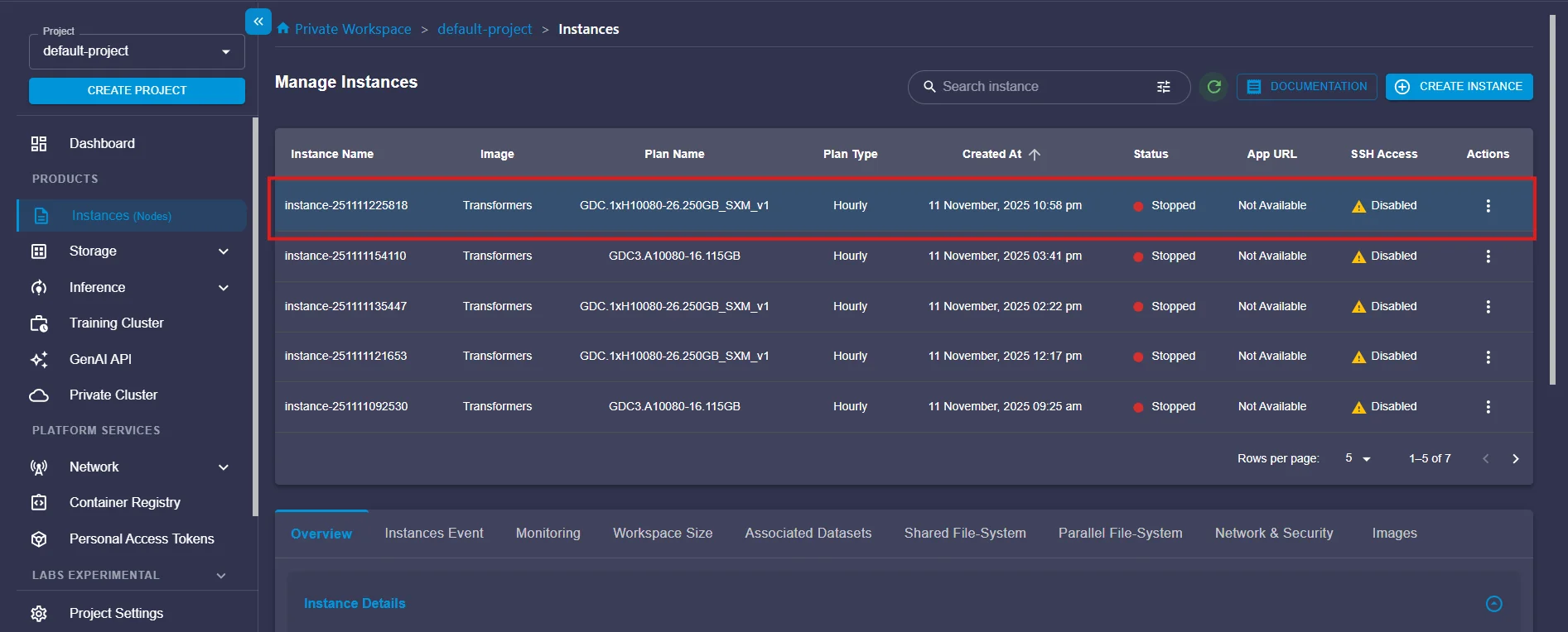
Once your instance status shows as Running, it's time to connect. You've got two great options:
-
SSH: This is the standard for most development. You can use the provided SSH command directly in your local terminal.
Pro-Tip: For the best experience, connect your favorite IDE (like VS Code with the Remote - SSH extension) to the instance's IP address. This gives you a full-featured coding environment right on your powerful remote machine.
-
Jupyter Lab: For quick experimentation or notebook-based work, simply click the Jupyter link provided on the instance details page. This will open a complete Jupyter Lab interface directly in your web browser—no local setup needed.
The Experiment: A Single Script for QAT vs. PTQ
Theory is great, but let's see the code. To fairly compare PTQ and QAT, I created a single training script that can run both experiments. The full script is available on GitHub and the trained models are on Hugging Face.
Here's the setup:
- Model: unsloth/Qwen3-4B-Instruct-2507 (a 4B parameter model from the Qwen3 family, optimized by Unsloth).
- Dataset: mlabonne/FineTome-100k (a high-quality, 100k-sample subset of the FineTome dataset).
- The Goal: Fine-tune this model on our dataset using two different methods, then benchmark the results.
- Experiment 1 (PTQ): Fine-tune in full precision (
BF16), then quantize to 4-bit after training. - Experiment 2 (QAT): Fine-tune while simulating 4-bit quantization.
- Experiment 1 (PTQ): Fine-tune in full precision (
The Script Walkthrough
Step 1: Configuration
The most important part of the script is this single flag. It controls whether we run the PTQ or QAT experiment.
QUANTIZATION_TYPE = "PTQ" # Options: "PTQ" or "QAT"

RUN_NAME = "Qwen3_4B_" + QUANTIZATION_TYPE
wandb.init(project = "QuantizationTraining", name = RUN_NAME)
This QUANTIZATION_TYPE variable will change our model setup and quantization steps later on.
Step 2: Load Model (in Full Precision)
Load our model using Unsloth's FastLanguageModel.
# Load the Model and Tokenizer
model, tokenizer = FastLanguageModel.from_pretrained(
    model_name = "unsloth/Qwen3-4B-Instruct-2507",
    max_seq_length = 2048,
    load_in_4bit = False,    # <-- Key!
    load_in_8bit = False,    # <-- Key!
    full_finetuning = False,
)
Important Note: This might seem counter-intuitive! Why are we setting
load_in_4bit = False?It's because we need to fine-tune the model first.
- For QAT, we load in full precision (
BF16by default on new GPUs) and let Unsloth simulate 4-bit during training.- For PTQ, we must train in full precision to create our baseline, which we'll quantize later.
Step 3: Add LoRA Adapters
This is where the paths for QAT and PTQ truly diverge. We use Unsloth's get_peft_model to add LoRA adapters. Pay close attention to the qat_scheme parameter.
# Add LoRA Adapters
model = FastLanguageModel.get_peft_model(
    model,
    r = 16,
    target_modules = ["q_proj", "k_proj", "v_proj", "o_proj",
                      "gate_proj", "up_proj", "down_proj",],
    lora_alpha = 32,

    # This is the magic line!
    qat_scheme = "int4" if QUANTIZATION_TYPE == "QAT" else None,

    use_gradient_checkpointing = "unsloth",
    random_state = 3407,
)
If our QUANTIZATION_TYPE is set to "QAT", Unsloth and torchao automatically inject "fake quantization" modules into our model. This is what makes it "Quantization-Aware." If the type is "PTQ", qat_scheme is None, and it performs a standard BF16 LoRA fine-tuning.
Step 4: Data Preparation and Training
We load the mlabonne/FineTome-100k dataset, apply the Qwen3 chat template, and set up the SFTTrainer from TRL.
# Load training dataset
dataset = load_dataset("mlabonne/FineTome-100k", split = "train")

# Apply chat template
def formatting_prompts_func(examples):
   convos = examples["conversations"]
   texts = [tokenizer.apply_chat_template(convo, tokenize = False, add_generation_prompt = False) for convo in convos]
   return { "text" : texts, }

dataset = dataset.map(formatting_prompts_func, batched = True)

# Train the model
trainer = SFTTrainer(
    model = model,
    tokenizer = tokenizer,
    train_dataset = dataset,
    args = SFTConfig(
        dataset_text_field = "text",
        per_device_train_batch_size = 4,
        gradient_accumulation_steps = 4,
        num_train_epochs = 1,
        learning_rate = 2e-5,
        logging_steps = 50,
        optim = "adamw_8bit",
        seed = 3407,
        report_to = "wandb",
    ),
)
trainer_stats = trainer.train()
After this step, trainer.train() runs. The QAT model trains a bit slower because of the extra quantization simulation, but it's learning how to be 4-bit. The PTQ model just trains normally. QAT model training took approximately 4 hrs. to train while PTQ model took 2 hrs. only.
Step 5: Applying Quantization
Here's how we finalize the models.
Path 1: Post-Training Quantization (PTQ)
If QUANTIZATION_TYPE == "PTQ", our training just finished. We now have a BF16 model with LoRA adapters. We must:
- Merge the LoRA adapters into the base model to get a full, fine-tuned
BF16model. - Save this full model.
- Reload the saved model and apply 4-bit quantization now.
# Check our flag
if QUANTIZATION_TYPE == "PTQ":

    # 1. Merge and save the full-precision model
    basline_name = RUN_NAME.replace("PTQ", "baseline")
    merged_model = trainer.model.merge_and_unload()
    merged_model.save_pretrained(f"./{basline_name}")
    tokenizer.save_pretrained(f"./{basline_name}")

    # 2. Define our 4-bit PTQ config from torchao
    quant_config = Int4WeightOnlyConfig(group_size=128,
                                        int4_packing_format="tile_packed_to_4d")
    quantization_config = TorchAoConfig(quant_type=quant_config)

    # 3. Reload the model and apply 4-bit quantization
    model = AutoModelForCausalLM.from_pretrained(
        f"./{basline_name}",
        device_map="auto",
        torch_dtype=torch.bfloat16,
        quantization_config=quantization_config
    )
    tokenizer = AutoTokenizer.from_pretrained(f"./{basline_name}")
Path 2: Quantization-Aware Training (QAT)
If QUANTIZATION_TYPE == "QAT", our model is already "aware." We don't need to merge and reload. We just tell torchao to convert the "fake quantized" modules into real 4-bit quantized layers.
# Check our flag
if QUANTIZATION_TYPE == "QAT":
    # Just convert the already-trained model!
    quantize_(model, QATConfig(step = "convert"))
That's it. It's a single line. This step swaps the simulation-time modules for fast, 4-bit inference-time modules.
Step 6: Save the Final Model
Finally, we save our quantized model. The QAT model requires a special save function from torchao.
if QUANTIZATION_TYPE == "QAT":
    model.save_pretrained_torchao(
        RUN_NAME,
        tokenizer,
        torchao_config = model._torchao_config.base_config,
    )
else: # PTQ
    model.save_pretrained(f"./{RUN_NAME}")
    tokenizer.save_pretrained(f"./{RUN_NAME}")
Now we have three different models, ready for benchmarking.
- Baseline model before applying PTQ (16 bit).
- Post Training Quantized model (4 bit).
- Quantization aware trained model (4 bit).
Model Evaluation on Multiple Benchmarks
To really know if our training and optimization actually helped, we need to test it with standardized benchmarks.
Think of these tests as a "report card" for the model. They move us past vague feelings and give us cold, hard numbers, showing us exactly where the model shines and where it struggles. To get a complete picture, we used two very different tests:
The Benchmarks We Picked
1. MMLU-Pro
MMLU-Pro is a collection of over 12,000 extremely tough, multiple-choice questions.
- The questions are pulled from 14 professional and academic domains, including law, medicine, advanced mathematics, philosophy, and engineering.
- This test shows if our model can reason like a specialist, not just repeat facts. Can it solve a complex legal problem or understand an advanced engineering concept?
- The Score: It's a simple Accuracy (%). You want the highest score possible. Higher is better.
2. WikiText
WikiText uses the WikiText-103 dataset, which is a high-quality collection of over 100 million words from verified, "good" Wikipedia articles.
- This benchmark measures the model's core grasp of the English language. How good is it at predicting the next word in a sentence? This tests its understanding of grammar, context, and common sense. A model that does well here is fluent and "understands" how sentences are built.
- The Score: It gives a score called Perplexity (PPL). This one is the opposite of MMLU: Lower is better. A low score means the model was "less surprised" by the text—its predictions were very accurate.
How to Run These Benchmarks with lm-eval
We didn't build our own testing setup from scratch—and you shouldn't either. We used the awesome open-source tool lm-evaluation-harness (everyone just calls it lm-eval) from EleutherAI.
There are some package incompatibility issues with torch, torchao, vllm and these will likely get resolved as some folks have already reported them on the official torchao GitHub repo. Follow the steps below to run the torchao 4-bit model inference smoothly without those issues.
Step 1: Create Python env and activate it
python -m venv qat-evalsource qat-eval/bin/activateStep 2: Install torch and torchao nightly index
pip install --pre torch torchvision torchaudio torchao --index-url https://download.pytorch.org/whl/nightly/cu128Step 3: Install vllm nightly wheel
pip install --pre vllm --extra-index-url https://wheels.vllm.ai/nightlyStep 4: Install Unsloth
pip install unslothStep 5: Clone the lm-eval repository
git clone https://github.com/EleutherAI/lm-evaluation-harness.git
cd lm-evaluation-harness
Step 6: Install the dependencies
pip install -e .Step 7: Run the WikiText Test
You're all set. Here's the command to run the WikiText benchmark. You can point it at a model you've got saved locally or any model on the Hugging Face Hub.
lm_eval --model hf \
    --model_args pretrained=jaytonde05/Qwen_4B_PTQ \
    --tasks wikitext \
    --device cuda:0
    --batch_size 1
So, what's all that code mean?
--model hf: Selects which model type or provider is evaluated.--model_args pretrained=...: This is where you point to your model.
- For a local model:
pretrained=./my-quantized-model- For a Hub model:
pretrained=jaytonde05/Qwen_4B_QAT--tasks wikitext: This is the key! We're telling it which test to run. (If you wanted MMLU-Pro, you'd put its task name here, like--tasks mmlu_pro).--device cuda:0: Select your GPU to use for evaluation.
Benchmark Results
We've completed the experiments, and it's time to see how our models performed. We're comparing three different versions:
- Baseline (BF16): Our original model, fine-tuned with LoRA in
bfloat16. This is our "full-precision" benchmark. - PTQ (4-bit): The Baseline model, but squished down to 4-bits after training (Post-Training Quantization).
- QAT (4-bit): Our new model, fine-tuned from the start using 4-bit Quantization-Aware Training (QAT).
Let's see if the extra effort of QAT paid off, starting with the MMLU-Pro accuracy test.
MMLU-Pro
MMLU-Pro is a tough benchmark that measures a model's reasoning and knowledge. For this test, a higher score is better.
| Model Version | MMLU-Pro Score (Higher is Better) |
|---|---|
| Baseline (BF16) | 0.4818 |
| PTQ (4-bit) | 0.4511 |
| QAT (4-bit) | 0.4903 |
Let's break down these results:
- The Baseline: Our original
BF16model set the bar with a score of 0.4818. - The Problem (PTQ): As expected, simply squishing the model with PTQ caused a performance drop. The score fell to 0.4511. This is the accuracy loss we need to fix.
- The Solution (QAT): The 4-bit QAT model didn't just fix the drop—it scored 0.4903, beating the original baseline by 1.76%!
The Accuracy and Recovery Calculation
This is the key takeaway. Let's look at it in two simple ways:
1. Performance vs. Original (QAT vs. Baseline)
This compares our final 4-bit model to the original full-precision model.
- Calculation:
((0.4903 - 0.4818) / 0.4818) * 100 - Result: Our 4-bit QAT model is 1.76% more accurate than the original
BF16model.
2. The "Recovery" Story (QAT vs. PTQ)
This tells us how well QAT fixed the specific problem caused by PTQ.
- Accuracy Lost by PTQ:
0.4818 - 0.4511 = 0.0307(This was the "problem") - Accuracy Gained by QAT:
0.4903 - 0.4511 = 0.0392(This is what QAT "fixed") - Recovery Percentage:
(0.0392 / 0.0307) * 100 =~127.7%
You read that right. QAT recovered over 100% of the lost accuracy plus gave us more 27%, smashing past the original baseline. This is a huge win.
WikiText Perplexity
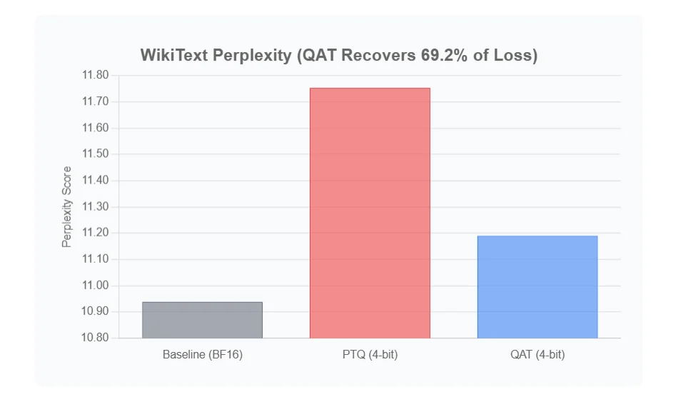
Next, we used WikiText to measure perplexity. Perplexity checks how well a model predicts the next word in a sentence. For this test, lower is better, as it means the model is less "perplexed" or confused.
| Model Version | Perplexity (Lower is Better) |
|---|---|
| Baseline (BF16) | 10.9391 |
| PTQ (4-bit) | 11.7545 |
| QAT (4-bit) | 11.1904 |
This benchmark tells a slightly different but equally important story:
- The PTQ model performed the worst, with the highest perplexity (11.7545).
- The QAT model (11.1904) landed right between the PTQ model and the Baseline.
It didn't beat the baseline here, but it dramatically improved on the PTQ model. Let's do the recovery math again.
The Recovery Calculation
-
Performance Gap to Fix: First, how much worse did PTQ do than the baseline?
11.7545 (PTQ) - 10.9391 (Baseline) = 0.8154This 0.8154 increase in perplexity is the "gap" we need to close. -
Performance Recovered: How much of that gap did QAT close?
11.7545 (PTQ) - 11.1904 (QAT) = 0.5641QAT clawed back 0.5641 points of perplexity. -
Percentage Recovered:
(0.5641 / 0.8154) * 100 =~69.2%
The QAT model closed 69.2% of the performance gap, bringing it much closer to the original baseline than the simple PTQ model.
QAT is a clear winner. On complex reasoning (MMLU-Pro), it didn't just recover the accuracy lost from 4-bit quantization—it actually exceeded the original baseline's performance. On a language modeling task (WikiText), it recovered over two-thirds of the performance hit.
This shows that "training-aware" quantization is a powerful technique to get small, fast models without sacrificing performance.
And the best part? These torchao-quantized models are fully compatible with high-performance inference engines like vLLM. You can take the QAT model we just trained, load it into vLLM, and get top-tier accuracy at top-tier speeds in production.
Conclusion
For years, using 4-bit quantization always meant making a compromise. We used it for the speed, but we had to settle for a noticeable drop in model accuracy.
Post-Training Quantization (PTQ) is fast, simple, and still has its place. If you have a fully-trained model and just need a "good enough" 4-bit version right now, it's a valid option.
But our experiment shows that Quantization-Aware Training (QAT) is clearly the superior approach.
By making the model "aware" of its 4-bit future during fine-tuning, the Unsloth and torchao stack delivered a model that:
- Recovered 69% of the accuracy lost by PTQ on a task like WikiText.
- Performed better than the original
BF16baseline.
Yes, QAT takes slightly longer to train due to the added simulation, but no need to do trade-off between speed and accuracy. You're investing a little more time in training to get a final model that is both fast and smart.
For any serious production use case where accuracy is non-negotiable, QAT should be your new default.
Get the Code
You don't have to take my word for it. All the code, benchmarks, and trained models are publicly available. I encourage you to run the notebook, test it on your own data, and see the results for yourself.
-
Full Training Script: GitHub Repo
-
Trained Models:
-
Wandb runs:
Happy quantizing!
References
- Quantization Aware training blog by unsloth : Quantization-Aware Training (QAT)
- TorchAO official git repo : TorchAO
- TorchAO INT4 PTQ receipe : Huggingface model repo
- MMLU-Pro git repo for installation and setup : MMLU-Pro